Mutation free energy calculations
A. Introduction
Now we are entering the realm of protein design. We will take a small protein
and try to make it better. Or at least more stable. In order to achieve that,
we are going to carry out "alchemical" mutations during the simulations and
compute the corresponding free energy changes. If we do this both in the
folded and unfolded states, and compute the difference between them, this
will yield us an estimate of the difference in stability between wild type
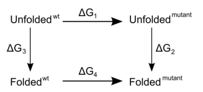
and mutant, as indicated in this thermodynamic cycle:
Experimentally, to address the same question, we would access the vertical
legs of the cycle and carry out folding/unfolding experiments to determine
ΔG3 and ΔG2. The difference ΔΔG =
ΔG3 - ΔG2 is then the difference in folding free
energy between wild type and mutant. In the simulations, this would be too
demanding, as even the folding time of a small peptide can be computationally
prohibitive, therefore preventing us from reliably obtaining the folding free
energies ΔG3 and ΔG2 directly from the
simulations for most peptides and proteins. However, we can relatively
accurately obtain the mutation free energies ΔG1 and
ΔG4 from "alchemical" mutations in which we morph one amino
acid into another and compute the according free energy change. If we do that
both in the folded and the unfolded states, we can make use of the fact that
the free energy is a state variable and therefore that the sum of all four
free energy values must be zero. Or, to put it differently, ΔΔG =
ΔG3 - ΔG2 = ΔG1 -
ΔG4. For the unfolded state, we do not really know what it
looks like. So we are going to assume that it can be modeled by a small piece
of unstructured peptide.
In the current tutorial we will focus on the simulation preparation of a folded protein,
however, an identical procedure can be applied to the short unstructed peptides as well.
In fact, the free energy differences for mutations
in GXG tripeptides can be precomputed for a given mutation library in a
specific force field.
Here you can find the precomputed ΔG values for GXG
tripeptides in several force fields.
Go back to Contents
B. Preparation
 We are now going to set up our first mutation simulation. The set up is a bit
different from a usual gromacs set up, as we use the
pmx package for
this, which is an add-on to gromacs. We prepared an example based on a small
protein minimal protein, to keep things simple and tractable. Of course, feel
free to mutate another protein, at the risk that the simulations will likely
take considerably longer. The next example assumes that you work with the
prepared "peptide.pdb". If not, please rename the filenames accordingly.
We are now going to set up our first mutation simulation. The set up is a bit
different from a usual gromacs set up, as we use the
pmx package for
this, which is an add-on to gromacs. We prepared an example based on a small
protein minimal protein, to keep things simple and tractable. Of course, feel
free to mutate another protein, at the risk that the simulations will likely
take considerably longer. The next example assumes that you work with the
prepared "peptide.pdb". If not, please rename the filenames accordingly.
First, let us have a close look at the structure and see which mutation you'd
consider to be potentially stabilizing:
pymol peptide.pdb
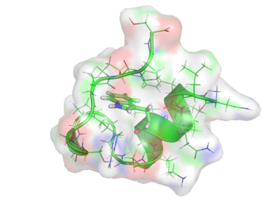
You will see that the peptide is folded around a central tryptophan
residue. It might be tempting to mutate this residue, but remember that a
larger perturbation will take longer to converge in the simulation, so a
smaller or more conservative change might be more promising. In addition, it
is recommended not to introduce mutations that introduce charge
changes. This is due to the fact that the buildup of a net charge during the
morphing simulations can lead to artifacts and longer convergence times.
To define where we want the mutation and to set up the morph
structure we will use pmx mutate.py function.
Prior to doing that, set the GMXLIB variable to point to the path containing mutation
libraries.
In case the paths are not yet properly set on the machine you are working on,
you will need to set GMXLIB manually.
Find out where the pmx source folder is and run
export GMXLIB=/home/bimbs/Downloads/pmx/pmx/data/mutff45
Also, it is convenient to add all the pmx scripts into your path.
To do that type:
export PATH=$PATH:/home/bimbs/Downloads/pmx/pmx/scripts
Now we are ready to perform the mutations. Run the mutate.py script:
mutate.py -f peptide.pdb -o mutant.pdb -ff amber99sbmut
Choose the residue you want to mutate and what you want to mutate it into.
Note that, as is frequently done in experiments, an alanine scan might be a
good starting point to identify promising locations.
Also, you may consider selecting a mutation for which a tripeptide value has already
been precomputed.
Once a mutation has been chosen, create a corresponding topology:
gmx pdb2gmx -f mutant.pdb -o conf.pdb -ff amber99sbmut -water tip3p
Here, the force-field used needs to be consistent with the force-field choice
from the previous step (amber99sbmut in this case).
We now have to post-process the topoloogy to add the morphing parameters:
generate_hybrid_topology.py -p topol.top -o newtop.top -ff amber99sbmut
In fact, these three steps of amino acid mutation and hybrid topology generation
could also have be carried out via a web-based interface.
Now we are ready to set up the simulation. First, we need to define a
simulation box:
gmx editconf -f conf.pdb -o box.pdb -bt dodecahedron -d 0.9
and we fill it with water:
gmx solvate -cp box -cs spc216 -o water.pdb -p newtop
To prepare the first energy minimization download the em.mdp file and run:
gmx grompp -f em.mdp -c water.pdb -p newtop.top
If you looked carefully, you'll see that grompp warned that the system carries
a net charge. In order to avoid artifacts due to a periodic charged system, we
add a chloride atom:
gmx genion -s -nn 1 -o ions.pdb -nname CL -pname NA -p
newtop.top
and select "13" as solvent group, so a water molecule can be replaced with a chloride ion. Now we can prepare for the energy minimization again:
gmx grompp -f em.mdp -c ions.pdb -p newtop.top -maxwarn 1
and carry out the actual energy minimization:
gmx mdrun -v -c em.pdb
Before we can set up the free energy calculation, we'll equilibrate the system
by running a short simulation of the wild type peptide (eq.mdp
file for equilibration):
echo 0 | gmx trjconv -s topol.tpr -f em.pdb -o em.pdb -ur compact -pbc mol
gmx grompp -f eq.mdp -c em.pdb -p newtop.top
gmx mdrun -v -ntomp 2 -nice 0 -c eq.gro
Note that you can also use more (virtual) cores for the simulation by
providing a larger number after -ntomp.
Now we are ready to do the actual free energy calculation. Please have a look
at the MD parameter file md.mdp. You will find a section
called "Free energy control" where you will see that free energy is switched
on, the initial lambda is chosen as zero, and that delta-lambda (per MD step)
is set such that at the end of the simulation lamda is at 1. Therefore, we are
using the "slow growth" method here. Now start the actual simulation.
gmx grompp -f md.mdp -c eq.gro -p newtop.top
gmx mdrun -v -ntomp 2 -nice 0 -c md.gro
Again, This will take a while. Nevertheless, the number of steps defined in
"md.mdp" corresponds to only 100 ps, which is too short to expect a converged
result, and therefore for an accurate free energy estimate. Therefore, to
assess convergence, we suggest to carry out two validation steps:
- make the simulation two, five or ten times longer (or shorter) and check
if you arrive at the same result.
- do the backward transition and check if you get the same result (but then negative).
Using the approach outlined above, try to find a reasonable balance between
computational effort and accuracy. Using the identified scheme, devise
a scheme to systematically identify mutations that stabilize the folded
structure of the peptide.
Go back to Contents
C. Free energy estimation
Slow growth thermodynamic integration (TI) approach relies on an assumption that during a transition
the system remains in a quasi-equilibrium state.
Therefore, integration over the dH/dl curve directly yields a difference
in free energy.
We have prepared a 10 ns forward and backward transitions of an S13A mutation
in the TRP cage protein.
Integration can be done using the gmx analyze tool. (Keep in mind that the integration
for lambda ranges from 0 to 1 for the forward direction and from 1 to 0
when integrating backwards)
gmx analyze -f dhdl.xvg -integrate
In practice, however, the slow growth TI is not frequently used.
An alternative method, that does not require an assumption of quasi-equilibrium during the alchemical transition
is the fast growth TI.
The fast growth TI approach relies on Jarzynski's equality (when transition is performed in one direction only)
or on the Crooks Fluctuation Theorem (when the transitions are performed in both directions).
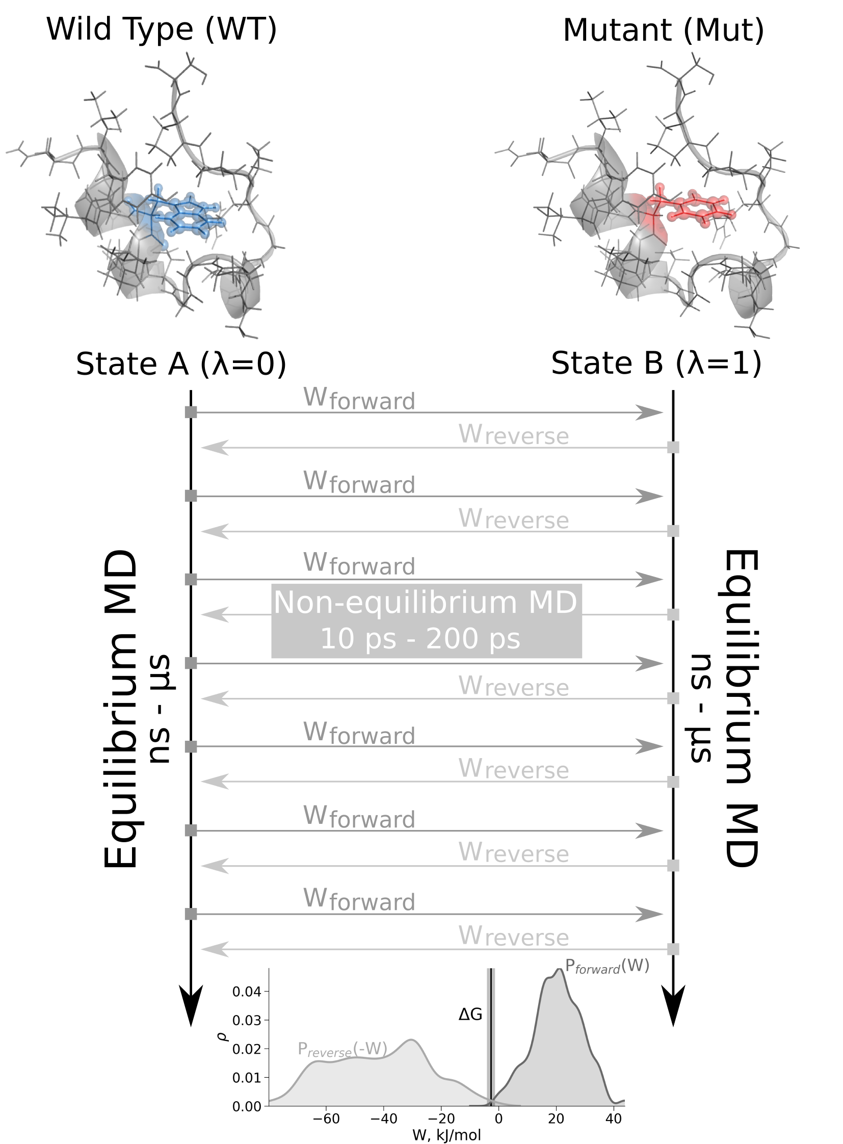
The schematic representation of the non-equilibrium alchemical free energy calculations is depicted on the right.
Here, free energy difference in the folded state of a protein is calculated.
Firstly, two independent equilibrium simulations need to be performed by keeping the system in its physical states: WT and mutant.
These simulations need to sufficiently sample the end state ensembles, as the free energy accuracy will depend on the sampling convergence.
Typically the equilibrium simulations are in the nanosecond to microsecond time range.
From the generated trajectories snapshots are selected to start fast (typically 10 - 200 ps) transitions driving the system
in the forward (WT to mutant) and reverse (mutant to WT) directions.
The work values required to perform these transitions are collected and the Crooks Fluctuation Theorem is
used to calculate the free energy difference between the two states.
The archive file S13A_fast_growth.tar.gz
contains two 10 ns simulation trajectories for the system in state A (eqA directory) and B (eqB directory).
(In case this file appears to be too large, you can download the file with analysis
folder only.)
From the trajectories 100 snapshots have been extracted and a fast 50 ps simulation has been performed
starting from each frame. During the simulation a system was driven from from state A to B (and vice versa)
in a non equilibrium manner and the dH/dl values were recorded.
pmx has utilities allowing to integrate over the multiple curves and subsequently estimate free energy differences
using several approaches: Crooks Gaussian Intersection, Bennet Acceptance Ratio or Jarzynski's estimator:
analyze_dhdl.py -fA eqA/morphes/frame*/dgdl.xvg -fB eqB/morphes/frame*/dgdl.xvg -t 300 --nbins 25
The free energy estimates are summarized in the file results.dat.
You can also investigate the individual work values for every transition in the forward (integ0.dat) and
backward (integ1.dat) directions. How do the non-equilibrium work values compare
to the quasi-equilibrium slow growth work estimates?
The script also produces several plots facilitating analysis of the work distributions.
So far we have investigated only one part of the cycle involving the folded protein.
To construct a double free energy difference the ΔG value for a mutation in the unfolded protein
(which we approximate by a GXG tripeptide) is needed.
The results for the A2S mutation in the tripeptide can be found here.
The final ΔΔG value will indicate whether the mutation is stabilizing the protein in its folded state.
Experimental measurements suggest that S13A mutation is mildly stabilizing (1.8 kJ/mol)
Barua et al, 2008.
Go back to Contents
D. Further steps
Depending on time and interests, address one or more of the following
questions:
- Now we have some data on which mutations work stabilizing or
destabilizing. But do we also understand why? Is it a particular interaction
in the folded state that was modified? Was the effect as predicted/expected?
What about entropic effects? Hint: use g_energy to look at individual energy
terms and interactions. Also take a close look at the simulation structures
to look at structural changes and specific interactions, like hydrogen bonds.
- In addition to the slow growth scheme applied above, frequently used
alternatives include so called discrete TI (DTI) and non-equilibrium methods
such as the Crooks Gaussian Intersection (CGI) method based on the Crooks
fluctuation theorem. If you are interested to try out one of those methods,
discuss with the supervisors how such a simulation could be set up.
- In principle, it should also be possible to sample the vertical legs of
the thermodynamic cycle above, by simulating the actual folding/unfolding
equilibrium of the peptide. Although the folding time of the peptide is
multiple microseconds, and thereforethe spontaneous folding is not
accessible within the time of the course, we can still think about
simulation strategies to study enforced unfolding or also folding
studies. If you want to try this, let one of the supervisors know and
discuss your plans!
- In addition to the peptide studied here, it is alo highly interesting to
study the stability of the major secondary structure elements: alpha helices
and beta sheets. Therefore, if you're interested to investigate those,
identify a model alpha-helix of beta hairpin from the Protein Data Bank and
see if you can increase its stability!
Go back to Contents
Further references:
Books:
- Editors: Chipot C. , Christophe A. et al., Free Energy Calculations , Springer Series in Chemical Physics, Vol. 86, [link] .
- Vytautas Gapsys, Servaas Michielssens, Jan Henning Peters, Bert L. de Groot, Hadas Leonov. Calculation of Binding Free Energies. Molecular Modeling of proteins: 2nd edition. Book Series: Methods in Molecular Biology 1215: 173-209 (2015) [link]
Advanced reading:
- R. W. Zwanzig, High Temperature Equation of State by a Perturbation Method. I. Nonpolar Gases J. Chem. Phys. 22: 1420 (1954). [link]
- Goette M, Grubmuller H, Accuracy and convergence of free energy differences calculated from nonequilibrium switching processes. J. Comp. Chem. 30: 447-456 (2009). [link]
- Gapsys V, Michielssens S, Seeliger D, and de Groot BL pmx: Automated protein structure and topology generation for alchemical perturbations. J. Comp. Chem. 36:348-354 (2015) [link]
- Vytautas Gapsys, Servaas Michielssens, Daniel Seeliger and Bert L. de Groot. Accurate and rigorous prediction of the changes in protein free energies in a large-scale mutation scan. Angew. Chem. Int. Ed. 55: 7364-7368(2016) [link]
- Seeliger D, and de Groot BL Protein thermostability calculations using alchemical free energy simulations. Biophys. J. 98:2309-2316 (2010) [link]
Go back to Contents