Ligand modification free energy calculations
A. Introduction
In this tutorial we will use non-equilibrium free energy calculation setup
to estimate relative free energy difference between two ligands bound to thrombin.
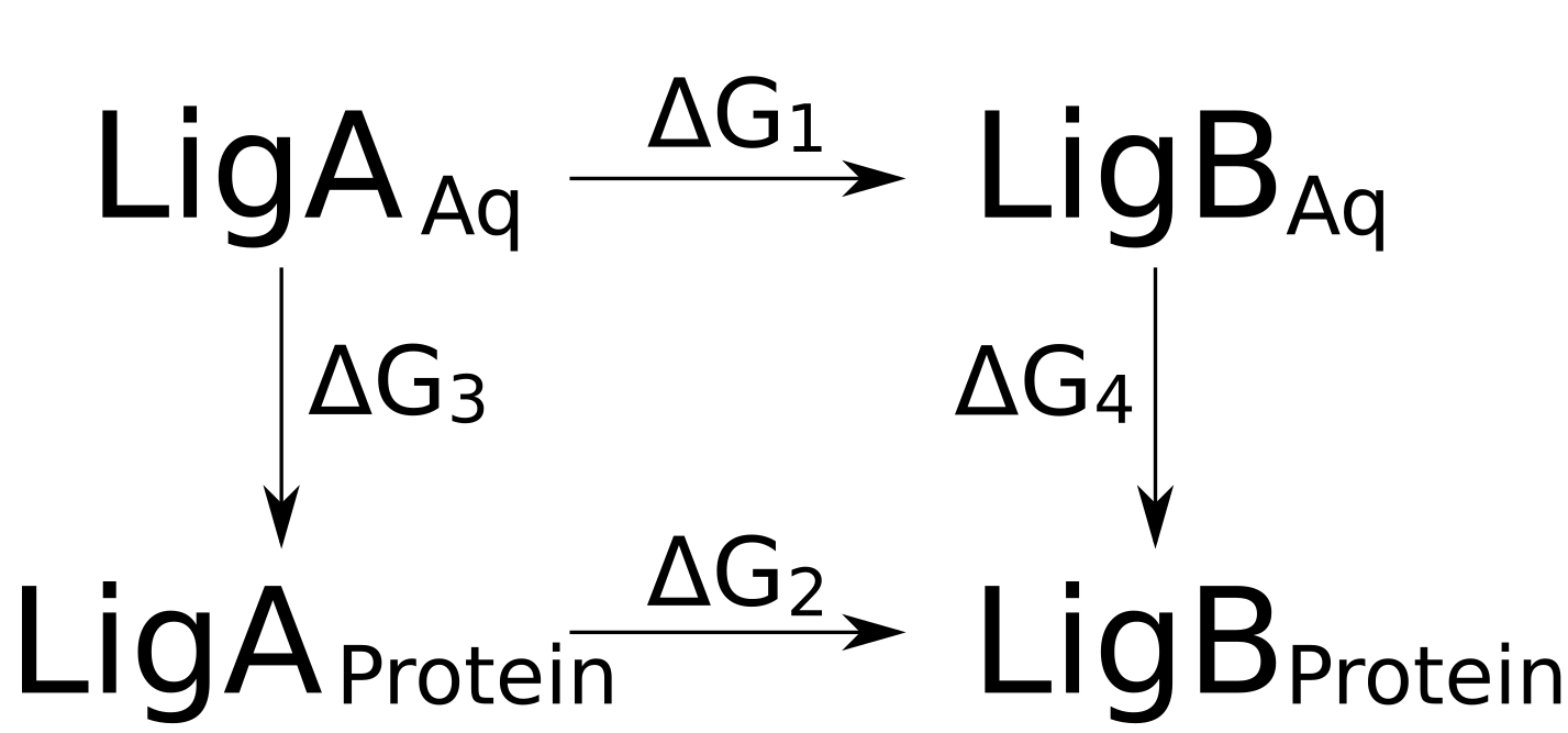
The double free energy difference can be expressed based on the thermodynamic cycle
depicted below:
In this scenario we are interested in obtaining the difference between the binding
free energies for the ligands B and A, i.e. ΔG4 - ΔG3.
However, converged sampling of these binding/unbinding events is computationally expensive.
We can rewrite the double free energy:
ΔΔG = ΔG4 - ΔG3 = ΔG2 - ΔG1
This way we replace the expensive sampling of the ligand binding/unbinding with a more
feasible alchemical ligand morphing from state A to B.
This alchemical modification we will be performed in a non-equilibrium manner.
We will use pmx to setup the required structures and topologies for the transitions.
For the ligand structure handling pmx relies on the rdkit package.
The topology generation for the ligand is not covered by the tutorial, i.e. we start at the step where
the ligand is already parameterized.
However, the process of initial ligand topology generation will be demonstrated in the introductory lecture.
B. Hybrid structures/topologies
 Firstly, we will generate hybrid structures and topologies for the subsequent simulations.
In the current tutorial we will consider two ligands from a set described in
this publication: ligands 1a and 5 depicted in Figure 1.
For both molecules the topologies have already been prepared following the standard procedure
for the generalized Amber force field (GAFF):
lig_1a and lig_5.
In the folders you will find a ligand structure file in .pdb format and two topology files: MOL.itp and ffMOL.itp.
MOL.itp contains information about atoms, bonds, angles and dihedrals, while atom types (van der Waals parameters)
are separated into ffMOL.itp file.
For further use it is convenient to merge both atom type ffMOL.itp files into one
(one_ff_file.py script will perform the merging):
Firstly, we will generate hybrid structures and topologies for the subsequent simulations.
In the current tutorial we will consider two ligands from a set described in
this publication: ligands 1a and 5 depicted in Figure 1.
For both molecules the topologies have already been prepared following the standard procedure
for the generalized Amber force field (GAFF):
lig_1a and lig_5.
In the folders you will find a ligand structure file in .pdb format and two topology files: MOL.itp and ffMOL.itp.
MOL.itp contains information about atoms, bonds, angles and dihedrals, while atom types (van der Waals parameters)
are separated into ffMOL.itp file.
For further use it is convenient to merge both atom type ffMOL.itp files into one
(one_ff_file.py script will perform the merging):
python one_ff_file.py -ffitp lig_1a/ffMOL.itp lig_5/ffMOL.itp -ffitp_out ffMOL.itp
To generate the hybrid structure and topology,
firstly, we will map the atoms of lig_1a and lig_5 to identify which atoms can be morphed
between the molecules.
This procedure will use pmx package.
Atom mapping is performed by the script atoms_to_morph.py:
python atoms_to_morph.py -i1 lig_1a/lig_1a.pdb -i2 lig_5/lig_5.pdb -o pairs.dat -alignment -H2H
The above procedure will perform the mapping based on the distances between atoms after an alignment.
Also, hydrogen atoms will be morphed into hydrogen atoms (in contrast to turning all hydrogens into dummies).
Feel free to play around with the mapping options, e.g. a flag "-mcs" will perform
a topology based mapping based on the maximum common substructure of the ligands,
however, for the current ligand pair the outcome remains unchanged.
An output of this script is a score (out_score.dat) of the mapping: a number close to zero indicates that
the ligands in the pair are similar to one another and are suitable for an alchemical modification.
Another output is the actual mapping of the atoms: pairs.dat file.
Next, we will use the created atom mapping to generate the hybrid structure and topology for the ligand pair
(make_hybrid.py script):
python make_hybrid.py -l1 lig_1a/lig_1a.pdb -l2 lig_5/lig_5.pdb -itp1 lig_1a/MOL.itp -itp2 lig_5/MOL.itp -pairs pairs.dat -oa merged.pdb -oitp MOL.itp -ffitp ffmerged.itp -scDUMd 0.1
The newly created merged.pdb file contains the hybrid structure (notice a dummy atom at the end of the atom list in the merged.pdb).
The coordinates in merged.pdb are based on the first ligand provided to the script, i.e. lig_1a.
mergedB.pdb has the same atoms as merged.pdb, but the coordinates in it are based on lig_5.
The hybrid topology with all the parameters explicitly defined for both physical states is provided in the MOL.itp file.
Any dummy atoms required for the hybrid structure are defined in the ffmerged.itp topology file.
Let's merge this atom types file with the previously generated ffMOL.itp:
python one_ff_file.py -ffitp ffMOL.itp ffmerged.itp -ffitp_out ffMOL.itp
For the further simulations we will also require topology of the protein: thrombin.
We can obtain it by running the standard Gromacs tool pdb2gmx (we will use Amber99sb-star-ildn-mut force field):
gmx pdb2gmx -f thrombin.pdb -o thrombin_pdb2gmx.pdb -water none -ff amber99sb-star-ildn-mut
This command will generate a thrombin structure with hydrogen atoms added.
Also, three topology files will be created named topol_Protein_chain_*.itp for every protein chain in the structure file.
It is convenient to assemble all the required .itp files into .top files.
According to the thermodynamic cycle in the figure above, we will need to setup two different branches of simulations:
1) ligand in water and 2) ligand bound to the protein.
For both of these cases we have prepared the .top files already: top_water.top
and top_protein.top.
Having generated all the required topologies, allows us to follow the standard Gromacs simulation setup procedures in the next step.
C. Equilibrium simulations
The following simulation setup steps can be easily added into a script to have a convenient automated procedure.
However, in the current tutorial we will go over the steps explicitly to provide the full detailed picture of the setup.
Four sets of equilibrium simulations will be required: 1) ligand_stateA in water, 2) ligand_stateB in water, 3) ligand_stateA bound to the protein,
4) ligand_stateB bound to the protein.
Therefore, it is convenient to create 4 respective directories:
mkdir stateA_water
mkdir stateB_water
mkdir stateA_protein
mkdir stateB_protein
The solvated simulation boxes need to be prepared only for the "stateA" in water and protein.
For the "stateB" we will re-use the same simulation setup and simply change the state via .mdp parameters.
At first, place the hybrid ligand structure in a box:
gmx editconf -f merged.pdb -o stateA_water/box.pdb -d 1.5 -bt dodecahedron
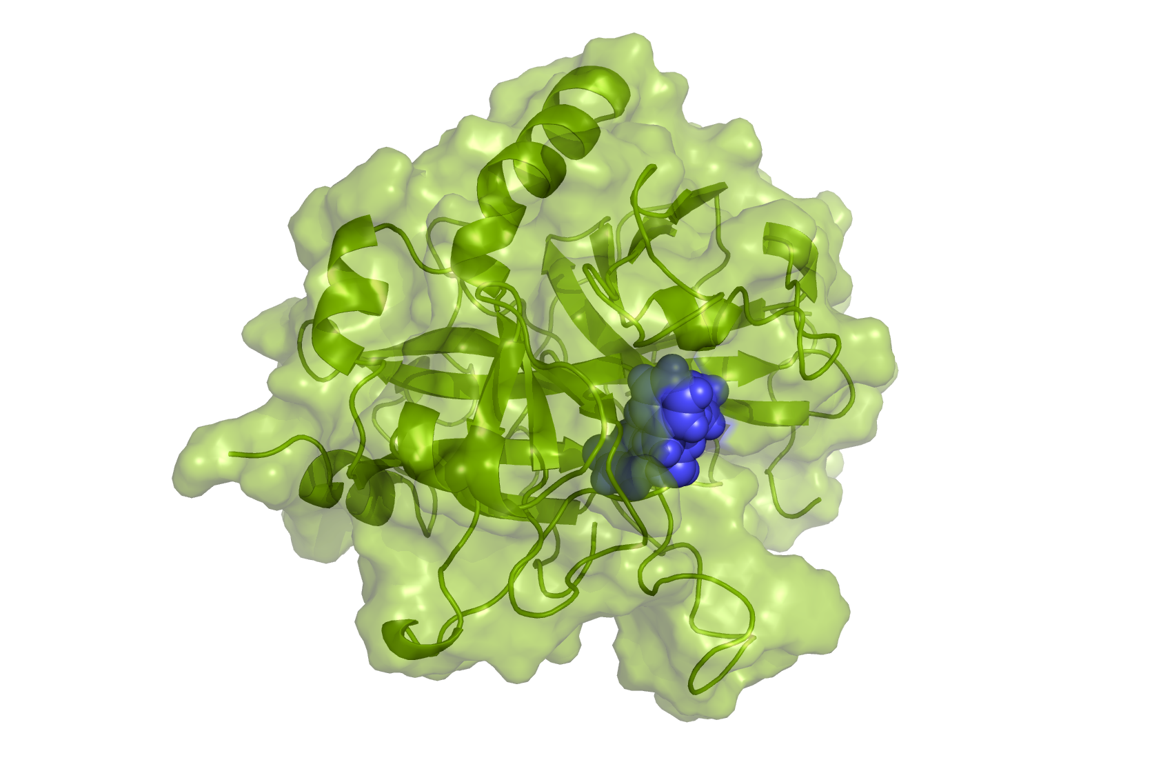
For the ligand bound to protein, we need to find the optimal pose for the ligand in the active site of thrombin.
There are several ways to do that: docking, MD simulations, alignment onto the experimentally determined structures.
In the current case, the initial ligand coordinates were built based on the crystallographic thrombin structure with
a bound inhibitor (pdb ID: 2ZDA).
This way, the hybrid structure is already in an appropriate pose.
Add ligand and protein together and generate the box:
awk '/ATOM/ {print $0}' thrombin_pdb2gmx.pdb merged.pdb > stateA_protein/thrombin_ligand.pdb
gmx editconf -f stateA_protein/thrombin_ligand.pdb -o stateA_protein/box.pdb -d 1.5 -bt dodecahedron
Solvate the systems:
gmx solvate -cs spc216.gro -cp stateA_water/box.pdb -o stateA_water/water.pdb -p top_water.top
gmx solvate -cs spc216.gro -cp stateA_protein/box.pdb -o stateA_protein/water.pdb -p top_protein.top
To add ions first download the .mdp files (they will also be used in the later setup steps).
Note that we will use non-standard ions reparameterized by
Joung and Cheatham: NaJ, ClJ.
The added ions neutralize the simulation box and reach 150 mM salt concentration.
gmx grompp -f mdp/emA.mdp -c stateA_water/water.pdb -o stateA_water/water.tpr -p top_water.top -maxwarn 2
gmx grompp -f mdp/emA.mdp -c stateA_protein/water.pdb -o stateA_protein/water.tpr -p top_protein.top -maxwarn 2
echo 4 | gmx genion -s stateA_water/water.tpr -neutral -conc 0.15 -o stateA_water/ions.pdb -nname ClJ -pname NaJ -p top_water.top
echo 15 | gmx genion -s stateA_protein/water.tpr -neutral -conc 0.15 -o stateA_protein/ions.pdb -nname ClJ -pname NaJ -p top_protein.top
Now we prepare files to start energy minimization:
gmx grompp -f mdp/emA.mdp -c stateA_water/ions.pdb -o stateA_water/em.tpr -p top_water.top -maxwarn 1
gmx grompp -f mdp/emB.mdp -c stateA_water/ions.pdb -o stateB_water/em.tpr -p top_water.top -maxwarn 1
gmx grompp -f mdp/emA.mdp -c stateA_protein/ions.pdb -o stateA_protein/em.tpr -p top_protein.top -maxwarn 1
gmx grompp -f mdp/emB.mdp -c stateA_protein/ions.pdb -o stateB_protein/em.tpr -p top_protein.top -maxwarn 1
To perform energy minimizations, enter the respective directory and run the command
(assuming the computer has at least 4 cores, otherwise adjust the -ntomp option):
gmx mdrun -s stateA_water/em.tpr -c stateA_water/emout.gro -v -ntomp 4 -ntmpi 1
gmx mdrun -s stateB_water/em.tpr -c stateB_water/emout.gro -v -ntomp 4 -ntmpi 1
gmx mdrun -s stateA_protein/em.tpr -c stateA_protein/emout.gro -v -ntomp 4 -ntmpi 1
gmx mdrun -s stateB_protein/em.tpr -c stateB_protein/emout.gro -v -ntomp 4 -ntmpi 1
Finally, prepare the equilibration runs. Usually equilibrium simulations should reach 10-1000 ns range,
however, for the purpose of current tutorial we will run only 100 ps equilibrium simulations:
gmx grompp -f mdp/eqA.mdp -c stateA_water/emout.gro -o stateA_water/eq.tpr -p top_water.top -maxwarn 1
gmx grompp -f mdp/eqB.mdp -c stateB_water/emout.gro -o stateB_water/eq.tpr -p top_water.top -maxwarn 1
gmx grompp -f mdp/eqA.mdp -c stateA_protein/emout.gro -o stateA_protein/eq.tpr -p top_protein.top -maxwarn 1
gmx grompp -f mdp/eqB.mdp -c stateB_protein/emout.gro -o stateB_protein/eq.tpr -p top_protein.top -maxwarn 1
Now perform "gmx mdrun" for each of the cases to run the simulations.
Even though the simulations are short (100 ps), on a slower machine the run may take some time.
Therefore we have performed the simulations in advance and you
can download the generated trajectories.
To further follow the tutorial, place the trajectories in the respective directories of your working folder.
D. Non-equilibrium transitions and analysis
The non-equilibrium transitions will be started from the structures extracted from the equilibrium simulations.
Let's extract snapshots from the pre-calculated trajectories:
echo 0 | gmx trjconv -s stateA_water/eq.tpr -f trajectories/stateA_water/traj_comp.xtc -o stateA_water/frame.gro -b 1 -pbc mol -ur compact -sep
echo 0 | gmx trjconv -s stateB_water/eq.tpr -f trajectories/stateB_water/traj_comp.xtc -o stateB_water/frame.gro -b 1 -pbc mol -ur compact -sep
echo 0 | gmx trjconv -s stateA_protein/eq.tpr -f trajectories/stateA_protein/traj_comp.xtc -o stateA_protein/frame.gro -b 1 -pbc mol -ur compact -sep
echo 0 | gmx trjconv -s stateB_protein/eq.tpr -f trajectories/stateB_protein/traj_comp.xtc -o stateB_protein/frame.gro -b 1 -pbc mol -ur compact -sep
Afterwards, for every starting structure generate a .tpr file for an alchemical transition from state A to B and vice versa.
Since there are 100 starting structures to go over, it may be convenient to place the following commands in a script
where a loop would run over the frames (we will use the first frame as an example):
gmx grompp -f mdp/tiA.mdp -p top_water.top -c stateA_water/frame0.gro -o stateA_water/tpr0.tpr -maxwarn 1
gmx grompp -f mdp/tiB.mdp -p top_water.top -c stateB_water/frame0.gro -o stateB_water/tpr0.tpr -maxwarn 1
gmx grompp -f mdp/tiA.mdp -p top_protein.top -c stateA_protein/frame0.gro -o stateA_protein/tpr0.tpr -maxwarn 1
gmx grompp -f mdp/tiB.mdp -p top_protein.top -c stateB_protein/frame0.gro -o stateB_protein/tpr0.tpr -maxwarn 1
Next, execute gmx mdrun command for every generated .tpr file.
Most likely, you would like to submit these jobs to run in parallel on a cluster.
Alternatively, you could run all these jobs sequentially on a fast machine (potentially using a GPU).
gmx mdrun -v -s stateA_water/tpr0.tpr -dhdl stateA_water/dhdl0.xvg -ntomp 4 -ntmpi 1
gmx mdrun -v -s stateB_water/tpr0.tpr -dhdl stateB_water/dhdl0.xvg -ntomp 4 -ntmpi 1
gmx mdrun -v -s stateA_protein/tpr0.tpr -dhdl stateA_protein/dhdl0.xvg -ntomp 4 -ntmpi 1
gmx mdrun -v -s stateB_protein/tpr0.tpr -dhdl stateB_protein/dhdl0.xvg -ntomp 4 -ntmpi 1
Executing all of the above commands one-by-one may seem tedious, however, it is easy to add all the steps
into one script. Here is an example of such a script written in python.
You can run the whole non-equilibrium calculation procedure simply by typing: python noneq_wrapper.py
Running all the transitions may take some time, therefore, we have performed the runs and collected the required
output.
To calculate the free energy difference between the states A and B for the ligand in water,
create an analysis folder (e.g. analysis_water), navigate to it and run the script:
analyze_dhdl.py -fA ../dhdlA_water/dhdl*xvg -fB ../dhdlB_water/dhdl*xvg -t 298
To analyze transitions for the ligand bound to protein, first create a respective analysis directory in
the main working folder and navigate to it. Then run the analysis script:
analyze_dhdl.py -fA ../dhdlA_protein/dhdl*xvg -fB ../dhdlB_protein/dhdl*xvg -t 298
The obtained results.dat files provide several free energy estimations with the respective errors.
One of the commonly used estimators is based on the maximum likelihood to observe the obtained work distributions
and is termed BAR (Benett Acceptance Ratio).
The difference between the BAR ΔG value for the ligand in protein and the value in water is exactly
the ΔΔG value we are interested in.
The calculated value is 0.26 kJ/mol, while the ITC value in the publication (Table 1)
is 0.4 kJ/mol.
To get a better feeling of the uncertainty associated with the calculated free energies investigate different estimators (CGI, BAR, Jarzynski),
error estimates, convergence measure, visually inspect work distributions and their overlap.
Go back to Contents
Further references:
- Gapsys V, Michielssens S, Seeliger D, and de Groot BL pmx: Automated protein structure and topology generation for alchemical perturbations. J. Comp. Chem. 36:348-354 (2015) [link]
- Vytautas Gapsys, Servaas Michielssens, Jan Henning Peters, Bert L. de Groot, Hadas Leonov. Calculation of Binding Free Energies. Molecular Modeling of proteins: 2nd edition. Book Series: Methods in Molecular Biology 1215: 173-209 (2015) [link]
Go back to Contents